
Ten Tests, Written Before the Code. The One That Failed Taught Me the Most
I wrote a finite element solver from nothing and pointed it at an answer known since 1898. It landed on 3.00002. Then a test I was sure would pass didn't, two explanations for why both collapsed, and a number the internet repeats confidently failed to reproduce.
The last article in this series asked what it takes to believe your own output when there is no experiment to check against. A black hole will not email you its spectrum.
This one is the opposite situation, and it turns out to be just as instructive. Here the exact answer is known — has been since 1898 — so "did I get it right?" is trivially checkable. Which means the interesting question changes. It stops being is the number right and becomes what would have caught me if it weren't.
So I did something I had not done before: I wrote the acceptance tests, with their pass thresholds, into an audit file before writing a line of the solver. Ten of them. Then I built the thing and ran them.
Nine passed. This article is mostly about the tenth.
The problem, and the one rule
Stretch a plate with a circular hole in it. The stress at the edge of the hole is exactly three times the stress far away — independent of the material, independent of the hole size, independent of how hard you pull. Kirsch published it in 1898.
The rule I set myself: the code is given the geometry, the elastic constants and the load, and never the number three.
That is easy to say and easy to cheat, so I made it checkable rather than asserted: grep the source for the target value and the only hits are a coefficient inside the analytic stress formula, a radius range in a sampling routine, and the comparison at the very bottom of the reporting block, after every number has already been computed. The mesher, the assembler, the solver and the stress recovery never see it.
No FEA library. No scipy — it isn't installed on this machine, which removed the temptation at the source. The Delaunay mesher, the quadrature, the elements, the assembly, the linear solver and the error norms are all hand-written.
Three things that had to be built first
The degenerate case was the common case
Delaunay triangulation by Bowyer–Watson has a well-known fragility: you insert a point, delete every triangle whose circumcircle contains it, and re-triangulate the cavity. If floating point marks one far-away triangle as "bad", the cavity stops being a simple polygon and the mesh is silently corrupt.
Textbooks treat that as a rare accident. On this problem it is the default: every node on the hole boundary lies exactly on one circle, so exact co-circularity is the normal input, not the pathological one. The fix is to keep only the connected component of the bad set containing the seed triangle, which makes a non-simple cavity impossible however the ties break.
And then not to trust that either. The empty-circumcircle property is measured on every finished mesh, after four rounds of smoothing and re-triangulation. Worst violation across all five refinement levels: exactly zero.
Quadrature you construct instead of remember
Two earlier experiments of mine were bitten by constants recalled from memory rather than read from a source. A hard-coded symmetric quadrature rule for triangles is exactly that kind of constant — seven points and weights you copy from somewhere and never verify.
So the rules are built: tensor-product Gauss–Legendre nodes mapped onto the triangle through the Duffy transform, then verified against the exact monomial integral.
integral over T of xi^p eta^q dA  =  p! q! / (p+q+2)!

worst relative error: 4.6e-15
A solver checked against a different solver
The production path is a hand-rolled Jacobi-preconditioned conjugate gradient. On the coarsest mesh it agrees with a dense direct factorisation to 5e-14. Two independent methods, same answer. The largest system in the study is 21,220 degrees of freedom.
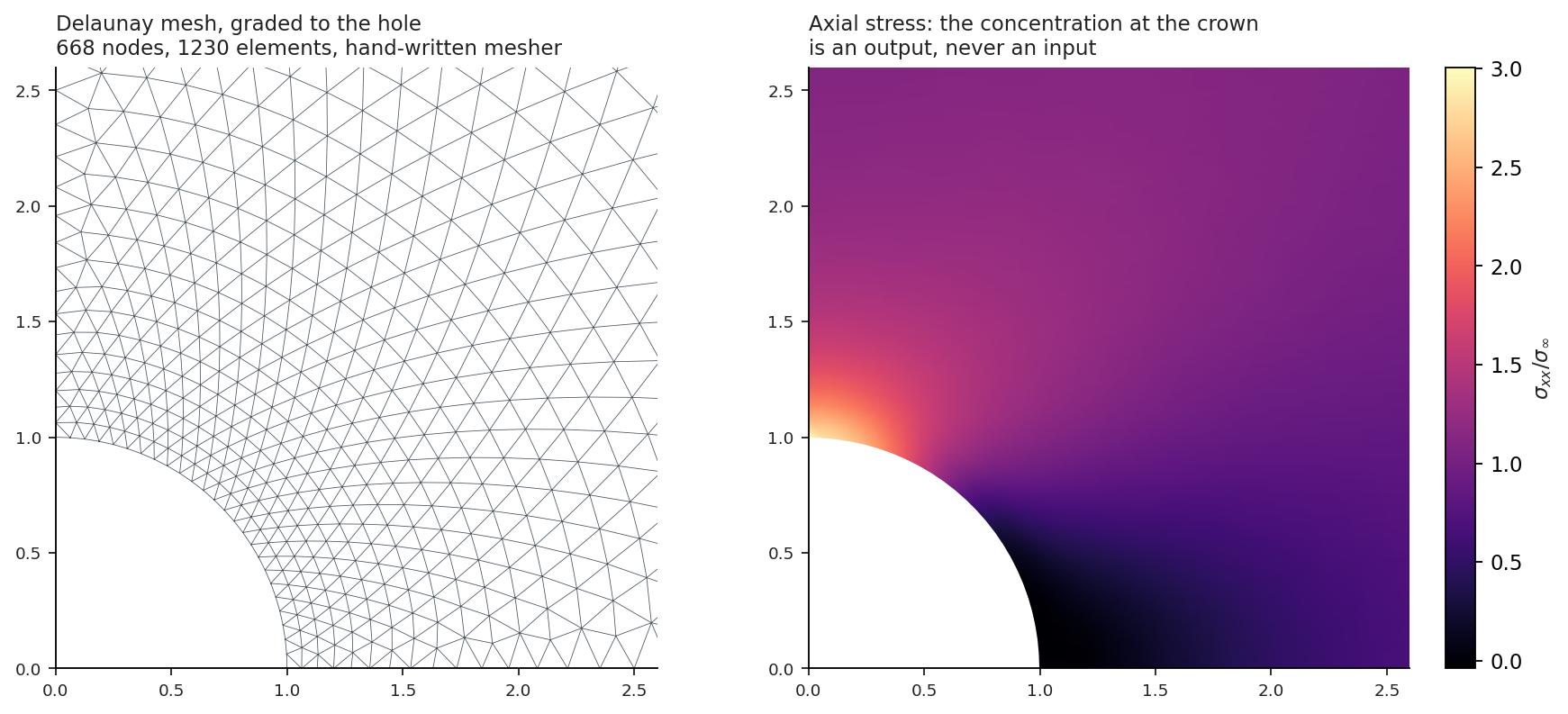
The mesh is graded so element size grows linearly with distance from the hole — neighbouring elements differ by a fixed ratio, so there are no size jumps, and refining scales a single number. On the right, the stress: bright at the crown where it reaches three, dark at the pole where a plate being pulled apart is in compression.
The test that was wrong, not the code
Before the interesting failure, a boring one that is worth more than it looks.
The patch test is the classical FEM sanity check: prescribe an exact polynomial displacement field on the boundary and the interior must reproduce it to round-off. I wrote one with an arbitrary quadratic field, ran it, and got an error of 8%.
My first instinct was that the quadratic elements were broken. They weren't. A patch-test field has to be an actual solution of the equations you are solving, and an arbitrary quadratic displacement produces a linear stress whose divergence is a non-zero constant — it needs a body force that isn't there. I was asking the solver to reproduce something that is not the answer, and it correctly refused.
Imposing equilibrium pins the field almost completely:
u = ( alpha x^2 , alpha q x y ) with q = -4/(1+nu)With that, it passes at 2e-14. The lesson is not about elasticity. It is that a failing test is a claim about two things, and the one you didn't write carefully is usually the test.
The gate that failed
Now the one I actually wrote this article for.
A curved boundary approximated by straight element edges is a classical "variational crime" — the domain you compute on is not the domain you meant. The standard remedy is to curve the elements, pushing mid-side nodes out onto the true circle. The standard claim is that skipping it costs you convergence order.
So I ran the quadratic elements twice, once curved and once with the hole deliberately faceted, to measure the cost instead of citing it. The prediction I registered in advance was deliberately weak — only that the energy-norm rate must drop by at least 0.25 — because the specific figure usually quoted for the loss came from a search summary rather than a paper I had opened, and I don't accept numbers on that basis.
| Run | L2 order | Energy order |
|---|---|---|
| Quadratic, curved hole | 3.249 | 2.013 |
| Quadratic, faceted hole | 2.045 | 2.031 |
| Order lost | 1.204 | −0.018 |
The crime costs a full order in L2 and nothing whatsoever in the energy norm. My gate asked about the energy norm. It failed.
I had two explanations ready, and both of them died.
That the global norm was hiding it. A graded mesh has far more elements out in the flat far field than around the hole, so a local error could plausibly be averaged away. Refuted: restricted to the ring around the hole where the crime actually happens, the energy rates are 1.992 curved against 2.014 faceted. No degradation there either.
That the loss is a Dirichlet phenomenon, since both curved boundaries here carry Neumann data. Refuted: re-running with the exact displacement prescribed on the curved outer boundary instead of a traction moves the answer by 0.001 of an order.
What survives is arithmetic, and it fits every number measured. The faceted domain perturbs the displacement at order h^2. That is worse than the h^3 the L2 error would otherwise reach, so it dominates and caps L2 at two. It is the same order as the h^2 energy error, so it changes only the constant — and the faceted energy error is indeed 5–7% larger at every level, on an identical slope.
Whether the widely quoted figure is wrong, or is right for a configuration I did not test, cannot be settled from here, and I am not settling it. I never opened the paper. That is precisely why the gate demanded a measurement instead of predicting a value — and why the honest output of this experiment is a measured number plus an admission, rather than a confirmation.
What the nine passing gates bought
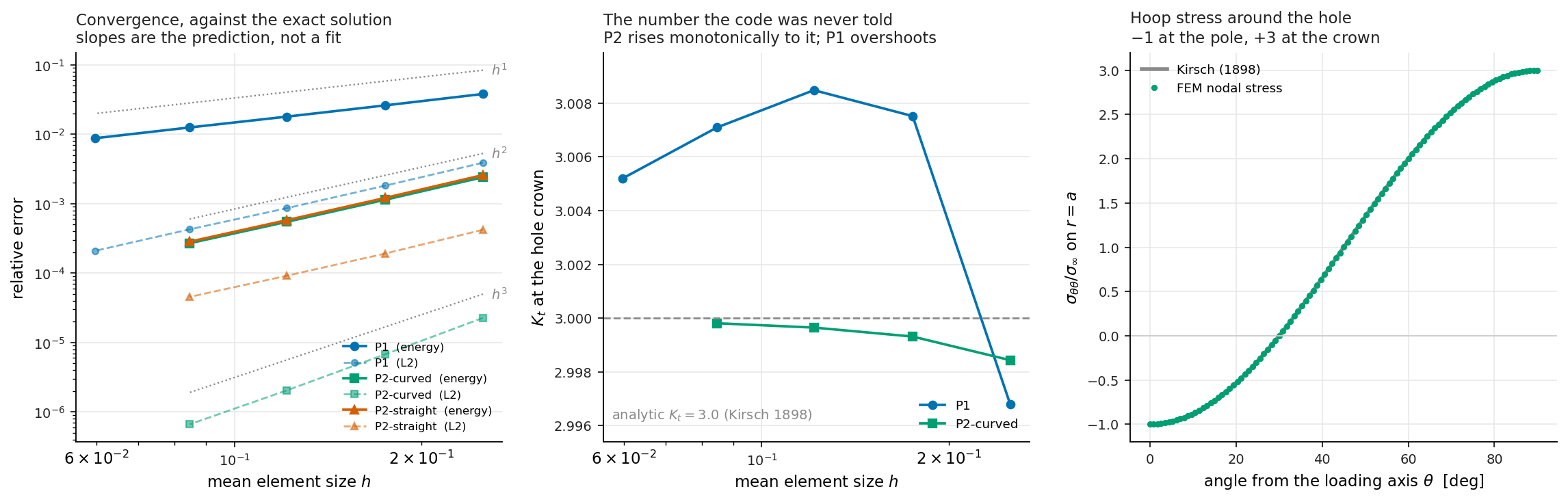
The concentration factor comes out at 3.00002 against an exact 3 — an error of 0.0005% — on a domain where the analytic field is the exact solution. A second, independent route, a finite plate extrapolated to zero width, gives 2.99970.
But the number is the least interesting result. Anyone can tune until one value matches. What cannot be faked is the rate: linear elements converge at 2.026 and 1.019 against a theoretical 2 and 1; quadratic elements at 3.249 and 2.013 against a theoretical 3 and 2. Two element families, four independent slopes, all landing on values the theory fixed in advance.
And one more piece of self-criticism that nobody forced: the quadratic L2 rate cleared its band by 0.001. A two-sided band was the wrong shape for a one-sided theorem, and that gate would have failed on a coarser mesh family. That is a flaw in the gate, not the code, and it is in the record.
What this is not
It is not new. Kirsch solved this in 1898, the convergence theory is textbook, and the plate-with-a-hole ships as a worked demo inside commercial FEA software. The literature audit that established all of that was written before any code and closed the project as research on its first page.
What was left is the only claim I make: implemented from first principles, and validated against analytic limits it was never fitted to.
It is also plane stress only, one geometry, one load case, static, small strain, two dimensions. The stress recovery is plain area-weighted nodal averaging, and the linear elements show no clean convergence order at the hole — which I have not fully explained. And I never read Kirsch's 1898 paper: the stress field came from a secondary source and the displacement field I derived myself, both checked numerically before being used as a ruler.
Reproduce it
One file, one command, about fifty seconds: python fem_003.py. It prints all ten gate results and writes its own evidence — the full gate log, convergence tables, hoop-stress data and both figures above. The archive, including the pre-registered audit, is deposited at doi.org/10.5281/zenodo.21892063.
If you take one thing from this: writing the tests down first cost me an afternoon and bought me the only genuinely interesting result in the project. A gate you write after seeing the number is not a gate. It is a description.